Using commands with Speech Recognition - Sixth Week

In my sixth week we considered submitting the project to Microsoft Open Source Challenge. I looked at the tools they had and found that the only one that was helpful for the project was the Speech API from Project Oxford. We could use speech recognition for voice commands in the Field Book app. That way the user would be able to take notes on the field easily and fast.

Project Oxford

This project from Microsoft Research is an Open Source set of APIs for vision, speech and language based on Artificial Intelligence. There is a code for speech recognition in Android, including a sample application that uses it. I downloaded it and ran it on my phone.The recognition works by sending an audio to a server, that after processing it responses with a list of 5 strings, each of one is a possible transcription of what the user said. Here is an example of how the code is:

MicrophoneRecognitionClient m_micClient;

SpeechRecognitionMode m_recoMode = SpeechRecognitionMode.ShortPhrase;

m_micClient = SpeechRecognitionServiceFactory.createMicrophoneClient(
        this,
        m_recoMode,
        language,
        this,
        subscriptionKey);

m_micClient.startMicAndRecognition(); 

The Activity has to implement the interface ISpeechRecognitionServerEvents in order to make the code above work.

There is also a tool called LUIS (Language Understanding Intelligent Service) that lets you build language models. This seemed to be a good thing to use because I wanted a specific language for the application (the language of the valid commands like "set height to 11"). But after testing it for a while, I realized that probably it wouldn't work. I was thinking that giving an input audio LUIS would give always a valid command as output, it turns out it doesn't. So I figured out I would have to make my own code that given a string returns a valid command.

Commands Design with Finite State Machine 

I looked at the problem of understanding a recognized speech as giving a list of words to a Finite State Machine (FSM) to process. If the FSM reads all the words that needs then is going to end on an acceptance state (the ones that has two circles around). That kind of state means a valid command in the application. This works better than simply comparing the string given by the speech recognizer because sometimes there might be words added by mistake. When working with Speech APIs you have to remember that the recognition may fail many times so your program must handle errors and try to fix them.

Diagram of a proposed Finite State Machine

Adding more classes - Fifth Week

In my fifth week I thought it was time to give the classifier something harder, so I added two more classes to the dataset. The classes were tomato and wheat. I thought that one application for the plant recognition could be that in the future robots would help farmers. They would have a semantic knowledge of plants so they would act different depending on that. For example if it’s wheat would give it some kind of fertilizer different that if it’s a tomato plant.

Training image of the wheat class

Then I trained with the new dataset and obtained bad results, around  60% of accuracy. To try to understand what was going on I implemented a confusion matrix, so that I could see specifically which classes were giving the biggest errors. I realized that classes like potato that had many images and descriptors did very good in testing but classes like cassava with fewer images and fewer descriptors. So probably the problem was that during K-Means the centers generated favor the classes that had more descriptors.

To fix this problem I decided to use the same amount of training and testing images for each class. So I selected 55 images for training and 30 for testing for each class in the dataset. I also changed the structure that the dataset had to have; now the training was separated from the testing image files in different folders inside the class, and now it wasn't necessary to store a dataset object, since the selection of the sets was fixed by where the image was.

Results with 5 classes

ORB Features

k = 32

Time for getting all the local descriptors of the training images was 00:00:02.476804.
Time for generating the codebook with k-means was 00:00:04.964310.
Time for getting VLAD global descriptors of the training images was 00:00:12.084776.
Time for calculating the SVM was 00:00:23.850120.
Time for getting VLAD global descriptors of the testing images was 00:00:06.300698.
Elapsed time predicting the testing set is 00:00:00.034392
Accuracy = 64.0.
Classes = ['cassava', 'pinto bean', 'tomato', 'wheat', 'potato']
Classes Local Descriptors Counts = [24507, 25720, 24192, 25232, 22500]
Confusion Matrix =
 [20  2  2  4  2]
 [ 3 17  1  7  2]
 [ 5  3 14  4  4]
 [ 2  0  1 26  1]
 [ 5  2  2  2 19]

k = 64

Time for generating the codebook with k-means was 00:00:09.258671.
Time for getting VLAD global descriptors of the training images was 00:00:17.179350.
Time for calculating the SVM was 00:00:46.991844.
Time for getting VLAD global descriptors of the testing images was 00:00:08.864136.
Elapsed time predicting the testing set is 00:00:00.065617
Accuracy = 65.3333333333.
Confusion Matrix =
 [19  3  6  1  1]
 [ 4 17  2  5  2]
 [ 4  3 15  6  2]
 [ 1  1  0 28  0]
 [ 4  3  3  1 19]

k = 128

Time for generating the codebook with k-means was 00:00:17.634565.
Time for getting VLAD global descriptors of the training images was 00:00:27.555537.
Time for calculating the SVM was 00:01:34.641161.
Time for getting VLAD global descriptors of the testing images was 00:00:14.336687.
Elapsed time predicting the testing set is 00:00:00.183201
Accuracy = 64.0.
Confusion Matrix =
 [21  2  3  1  3]
 [ 5 13  3  7  2]
 [ 4  4 14  5  3]
 [ 3  0  0 27  0]
 [ 2  4  2  1 21]

k = 256

Time for generating the codebook with k-means was 00:00:35.860902.
Time for getting VLAD global descriptors of the training images was 00:00:52.757244.
Time for calculating the SVM was 00:03:32.905707.
Time for getting VLAD global descriptors of the testing images was 00:00:26.958474.
Elapsed time predicting the testing set is 00:00:00.383407
Accuracy = 62.6666666667.
Confusion Matrix =
 [19  4  3  2  2]
 [ 5 15  2  6  2]
 [ 2  2 16  6  4]
 [ 2  0  0 28  0]
 [ 6  3  3  2 16]

SIFT Features

k = 32

Time for getting all the local descriptors of the training images was 00:00:31.042207.
Time for generating the codebook with k-means was 00:00:28.069662.
Time for getting VLAD global descriptors of the training images was 00:01:56.548077.
Time for calculating the SVM was 00:01:23.322534.
Time for getting VLAD global descriptors of the testing images was 00:00:57.089969.
Elapsed time predicting the testing set is 00:00:00.142989
Accuracy = 79.3333333333.
Classes = ['cassava', 'pinto bean', 'tomato', 'wheat', 'potato']
Classes Local Descriptors Counts = [73995, 79464, 38025, 86212, 28823]
Confusion Matrix =
 [22  2  3  0  3]
 [ 0 24  2  1  3]
 [ 0  1 23  3  3]
 [ 0  0  0 30  0]
 [ 1  6  1  2 20]

k = 64

Time for generating the codebook with k-means was 00:00:56.495541.
Time for getting VLAD global descriptors of the training images was 00:02:20.884382.
Time for calculating the SVM was 00:03:10.961254.
Time for getting VLAD global descriptors of the testing images was 00:01:07.280931.
Elapsed time predicting the testing set is 00:00:00.338773
Accuracy = 78.6666666667.
Confusion Matrix =
 [23  1  3  0  3]
 [ 1 24  2  1  2]
 [ 0  0 25  2  3]
 [ 0  0  1 29  0]
 [ 3  7  1  2 17]

k = 128

Time for generating the codebook with k-means was 00:48:26.116957.
Time for getting VLAD global descriptors of the training images was 00:03:2.914655.
Time for calculating the SVM was 00:06:52.834055.
Time for getting VLAD global descriptors of the testing images was 01:32:33.834146.
Elapsed time predicting the testing set is 00:00:0.620425
Accuracy = 77.3333333333.
Confusion Matrix =
 [23  1  3  0  3]
 [ 1 23  3  1  2]
 [ 0  1 25  1  3]
 [ 0  0  1 29  0]
 [ 1  9  3  1 16]

k = 256

Time for generating the codebook with k-means was 00:08:52.935980.
Time for getting VLAD global descriptors of the training images was 00:10:37.489346.
Time for calculating the SVM was 03:08:49.511758.
Time for getting VLAD global descriptors of the testing images was 00:05:28.551197.
Elapsed time predicting the testing set is 00:00:02.722835
Accuracy = 79.3333333333.
Confusion Matrix =
 [25  2  1  0  2]
 [ 0 25  2  1  2]
 [ 1  0 22  3  4]
 [ 0  0  0 30  0]
 [ 2  7  2  2 17]

Conclusion

I added more classes to the dataset to see how the classification performance would change. One of the important things I realized was that it's necessary to have similar amount of descriptors for each class if you are going to use K-Means (in our case we use it for a codebook from the Bag of Words technique). The best result went from 89.77% of accuracy to 79.33% but with different number of testing images for each case. It is also necessary to use always the same amount of testing images so that the comparison of the performances are more fair.

Confusion matrix for the best result obtained (SIFT k=32)

Looking in the Android Play Store I found applications that claimed to be able to recognize between 20.000 classes of plants. Using my method it would be very difficult to have that amount of classes.

First, it would need a lot of memory to store all the descriptors for each class. Using around 50 training images per class there would be about 20.000 descriptors per class and that's 400 M (million) vectors. Each vector uses at least 32 floating points number (of 32 bit = 4 bytes). So the data used for all the descriptors would be 32 x 4 bytes x 400 M = 51,200 M of bytes =51.2 x 10^9 bytes ~ 47.8 GB of RAM.

Second, it would take a lot of time to use K-Means for 400M vectors and to calculate an SVM for 20.000 classes usings 20.000 * 50 (number of training images) VLAD vectors.

Third, adding only 2 more classes there was a drop of 10% in the accuracy. Having more classes would make the codewords have less discriminating power because there would be many features and may be more similar from each other than with less classes.

When I looked at the reviews of that application many people complained about that the recognition didn't work. Someone said that even one of the most common plants wasn't recognized. Maybe it seems too difficult to have many possible classes, but now companies like Google have achieved very good performance with image recognition, for example in the Google Photos app one can search images using many categories like dog, beach, cascade, food, etc. So having robots that help in farming is possible and that could help feeding the growing population.

Classification of object in Android - Fourth Week

In my forth week I worked on a code for classifying images in Android. That is possible using the SVM calculated in the program in Python. The Support Vector Machine is saved in a file from Python and then is loaded on Android. It is also necessary to use OpenCV to get the local descriptors from the testing image and use the codebook to get the global descriptor. The codebook is also saved in a file from Python and loaded on Android using CSV format.

How to use OpenCV on an Android Activity

I created a new Activity on the Android project called TestActivity to make the debugging easier. It uses a picture that was already taken and stored in memory. To make an Activity work with OpenCV you can follow this tutorial
http://docs.opencv.org/2.4/doc/tutorials/introduction/android_binary_package/dev_with_OCV_on_Android.html.
In my case I added a LoaderCallback attribute to the TestActivity class:

private BaseLoaderCallback mLoaderCallback =

new BaseLoaderCallback(this) {

  @Override

  public void onManagerConnected(int status) {

      switch (status) {

          case LoaderCallbackInterface.SUCCESS: {

              Log.d(TAG, "OpenCV loaded");

          }

          break;

          default: {

              super.onManagerConnected(status);

          }

          break;

      }

  }

};

And this lines inside the onCreate() method:

// --------------------------------------------------------------------------

// OpenCVLoader

if (!OpenCVLoader.initDebug()) {

  mLoaderCallback.

onManagerConnected(LoaderCallbackInterface.INIT_FAILED);

} else {

mLoaderCallback.

onManagerConnected(LoaderCallbackInterface.SUCCESS);

}

// ---------------------------------------------------------------------------

Loading an OpenCV SVM on Android 

To use the SVM previously computed with Python it was necessary to do something triky. The SVM class has a function load(filename). The problem is that in Android filenames are not as easy as in a PC. You may have the file stored in external or internal memory, on the local folder of the app or in the res/raw/ directory of the source code. So I followed a sample from OpenCV Android, a project called face-detection. They store the model file in a /res/raw/ directory inside the source code and what they do is to open it and make a local copy of it. So when the load method is called it uses the local copy.

InputStream is = getResources().openRawResource(R.raw.lbpcascade_frontalface);

File cascadeDir = getDir("cascade", Context.MODE_PRIVATE);

mCascadeFile = new File(cascadeDir, "lbpcascade_frontalface.xml");

FileOutputStream os = new FileOutputStream(mCascadeFile);

byte[] buffer = new byte[4096];

int bytesRead;

while ((bytesRead = is.read(buffer)) != -1) {

  os.write(buffer, 0, bytesRead);

}

is.close();

os.close();

mJavaDetector = new CascadeClassifier(mCascadeFile.getAbsolutePath());

The method getAbsolutePath( ) is what you need as filename. After using that I was able to load the SVM and use it to predict the class of the image.

Result

Finally I also had to create a Vlad class to calculate the global descriptor for the image using the codebook and the local descriptors. After I did that I had all the elements to do a classification for the input image, which was an image of potatoes, and was correctly classified as that.

Results of classification - Third Week

In my third week I began testing the object classification code looking on accuracy and time of processing. These are the results:

Using ORB Features

For k (number of clusters, centers or codewords) = 64

Time for getting all the local ORB descriptors of the 356 training images was 00:00:09.533.
Time for k-means with ORB and k=64 was 00:00:16.574.
Time for getting VLAD global descriptors for k=64 and the 356 training images was 00:00:58.26.
Time for calculating the SVM for k=64 was 00:00:13.407.
Time for getting VLAD descriptors for k=64 and the 179 testing images was 00:00:28.784.
Time for classifying was 00:00:0.001.
Accuracy was 76.705%.

For k=128

Time for k-means with ORB and k=128 was 00:00:20.
Time for getting VLAD global descriptors for k=128 and the 356 training images was 00:02:24.651.
Time for calculating the SVM for k=128 was 00:00:34.648.
Time for getting VLAD descriptors for k=128 and the 179 testing images was 00:01:09.031.
Time for classifying was 00:00:0.001.
Accuracy was 80.114%.

For k=256

Time for k-means with ORB and k=256 was 00:00:59.893.
Time for getting VLAD global descriptors for k=256 and the 356 training images was 00:02:58.63.
Time for calculating the SVM for k=256 was 00:01:12.594.
Time for getting VLAD descriptors for k=128 and the 179 testing images was 00:01:27.856.
Time for classifying was 00:00:0.003.
Accuracy was 77.841%.

Using SIFT features

For k=64

Time for getting all the local SIFT descriptors of the 356 training images was 00:01:45.578.
Time for k-means with SIFT and k=64 was 00:01:33.133.
Time for getting VLAD global descriptors for k=64 and the 356 training images was 00:05:16.315.
Time for calculating the SVM for k=64 was 00:00:48.826.
Time for getting VLAD descriptors for k=64 and the 179 testing images was 00:02:05.115.
Time for classifying was 00:00:0.002.
Accuracy was 89.773%.

For k=128

Time for k-means with SIFT and k=128 was 00:02:51.927.
Time for getting VLAD global descriptors for k=128 and the 356 training images was 00:10:41.265.
Time for calculating the SVM for k=128 was 00:01:55.241.
Time for getting VLAD descriptors for k=128 and the 179 testing images was 00:04:17.92.
Time for classifying was 00:00:0.004.
Accuracy was 89.773%.

For k=256

Time for k-means with SIFT and k=256 was 00:05:23.914.
Time for getting VLAD global descriptors for k=256 and the 356 training images was 00:16:36.843.
Time for calculating the SVM for k=256 was 00:04:01.465.
Time for getting VLAD descriptors for k=256 and the 179 testing images was 00:05:41.41.
Time for classifying was 00:00:0.016.
Accuracy was 87.5%.

Results may be different using a SVM with other kernel like RBF. I only used a Linear kernel. Accuracy was calculated as number of correctly classified images / total number of images (in the testing set).

Object Classification - Second Week

About object classification

In my second week I started to developed a software for training an object classifier using images. The idea is that using an image as input, for example an image of potatoes the classifier would give the class of the image as output. That is done using Computer Vision and Machine Learning techniques. The Computer Vision part is that the program gets descriptors for the image and the Machine Learning part is that the descriptors are used to train a model that would classify another set of descriptors.

For example an article would be classified as sport, political news or other class depending on the words that are used. For example if an article has words like football, goals, points, team, etc. It would probably be an sports article. In that sense, the words are the descriptors of the article and they are different depending of the class they belong. A model is a rule for the set of descriptors that would take them and predict the class that is described by them.

About the program

I created a program on Python and OpenCV that uses ORB local descriptors, VLAD global descriptors and a SVM as classifier. It is free and can be downloaded on Github https://github.com/HenrYxZ/object-classification. To run it just use the command line

python main.py 

The program will look for a "dataset" directory inside the project folder. Then it will generate a Dataset object with the images found there. The images must be in a folder with the name of it class, for example all the images of potatoes must be in a "potatoes" folder. You don't have to divide the images between training and testing sets as the program will do that automatically with a random selection of 1/3 of the images for testing and the rest for training. Then the Dataset object will be stored in a file so that it can be used later and will have the information of which image is in which set and in which class.

After that the local descriptors for the training set are calculated. That is done using OpenCV functions. This tutorial shows how ORB descriptors are obtained http://opencv-python-tutroals.readthedocs.org/en/latest/py_tutorials/py_feature2d/py_orb/py_orb.html. I resize every image that has more than 640 pixels in one of its sides to have 640 pixels in its biggest size and conserving the aspect ratio to have a similar amount of local descriptors on every image. If an image has too high resolution it may give a lot of local descriptors and it would be difficult to have enough memory to store them all. If the dataset has too many images the program may crash because the computer may not be able to store all the descriptors in RAM memory.

An example of ORB descriptors found in a Cassava root image

When the local descriptors are ready a codebook is generated using K-Means (The technique is known as Bag of Words). A codebook is a set of vectors that theoretically have more descriptive power for recognizing classes. Those vectors are called codewords. For example a codeword for a car may be a wheel because cars have wheels no matter how different they are. The K-Means algorithm find centers that are representatives of clusters by minimizing the distance between the elements of a cluster to it center. The descriptors are grouped into k number of clusters (k is predefined) randomly at first but then in the groups that minimize distances. So for example for k=128 there are going to be 128 codewords which are vectors obtained by K-Means. A center is an average of descriptors and may have descriptors of different classes in its cluster space.

An example of a codebook with multiple words

Then for each image there is a global descriptor VLAD (Vector of Locally Aggregated Descriptors). This descriptor uses the local descriptors and the codebook to create one vector for the whole image. For each local descriptor in the image finds the nearest codeword in the codebook and adds the difference between each component of the two vectors to the global vector. The global vector is a vector of length equal to the dimension of the local descriptors multiplied by the number of codewords. In the program after the VLAD vector is calculated there is a square root normalization where every component of the global vector is equal to the square root of the absolute value of the previous component and then a l2 normalization where the vector is divided by its norm. That has had better results.

VLAD global descriptors

This global descriptors are given to a Support Vector Machine as input with the labels and it creates a model for the training set. I have used a Linear kernel but it's possible to use other kernels like RBF and maybe get better results. What the SVM does is to find decision lines or equations that are going to divide groups of vectors into one class or another. And it does that by maximizing the separation between decision lines and the minimizing the distance to the vectors of the same class. OpenCV comes with a SVM class that has a train_auto function that automatically selects the best parameters for the machine, and is what I use in the program.

After the SVM is trained the VLAD vectors of the testing images are calculated in the same way as in training and the global vectors are used with the SVM to predict their classes. Then the accuracy in the prediction is obtained by dividing the number of images that where correctly classified by the total number of images.

Implementation

I downloaded images from ImageNet of cassava roots, pinto beans and potatoes. And put them in a dataset folder inside the project. The best results where 80% of accuracy with a codebook of k=128.The training set where a total of 356 images and a testing set with 179 images total. The total time of processing was less than 3 minutes in a Intel I3 Ultrabook.

Color Segmentation - First Week

In my first week I downloaded the 1KK application and looked at the code. It is an Open Source Android project developed by Trevor Rife and is hosted on Github. The program works by taking a picture of seeds using a green background with blue circles. The circles are used to estimate the length per pixel of a picture by getting an average diameter of circle in pixel and knowing the real diameter of the circles. For getting the circles it's necessary to do a segmentation of the blue colors and for extracting the seeds from the image there is also a segmentation to remove the green and blue colors.

An example of an image taken with 1KK

The segmentation is done by using range of colors. The problem with this type of segmentation is that the ranges have to be found by experimentation. In the case of RGB colors they may be affected by lighting changes. For example a picture taken with a lot of light can have high values for RGB channels components but  with low illumination  the values would be low. So for the same range and the same objects the picture would give a different segmentation depending on the light. They use HSV color space for segmentation. To test the ranges predefined I used a software I created that lets you try with different color ranges and see the segmentation of the picture in real time (it also works with videos).

The software is free and is called color-range-selector. To run it you need to have Python and OpenCV installed. I used it on Windows 10 and this are the steps I followed to make it run:

How to install OpenCV for Python in Windows

1. First you need to install Python 2.7 by downloading and executing the msi installer. 
2. Then install the Python Development Tools for Windows that are available here http://aka.ms/vcpython27 .
3. After that you will be able to install the Numpy library for Python by running:

   pip install numpy

   in command line.
4.  Follow the instructions in this tutorial to install OpenCV for Python http://docs.opencv.org/master/d5/de5/tutorial_py_setup_in_windows.html .

How to install and use the color range selector

1. Download the project from Github by using the command line:

   git clone https://github.com/HenrYxZ/color-range-selector.git

2. Change the directory to the project:

   cd color-range-selector

3. Finally run the main program:

   python color_range_selector.py  

Selecting a range of color

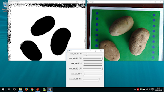
Segmentation using HSV range of colors with color-range-selector

The image shows the segmentation for using a range between (40, 0, 0) and (255, 255, 255) in HSV space. The result is capable to extract the green background and the blue circles. But for other image the ranges don't work.

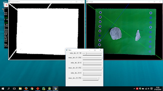
Testing a segmentation using HSV range and not working

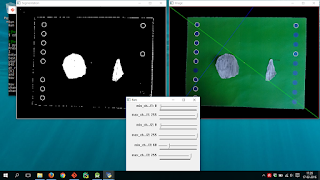
But using a BGR color range seems to work better in the second case. The idea is to use a high minimum value for the red channel. That is because both green and blue are far from the red in the BGR color space. This are the results using a range between (0, 0, 60) and (255, 255, 255):

Testing segmentation on BGR and working well

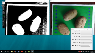
Segmentation on BGR with inferior results than HSV

In conclusion, HSV space may be used for segmentation with low change of hue. For example using seeds or potatoes with brownish hue works well, but the testing using papers of gray hue not. On the other hand, BGR lets use more different colors of seeds but the segmentation is affected by the illumination.

Introduction

Hi, I'm Hernaldo! The purpose of this blog is to document my work as a Research Intern at Texas A&M University. On 2015 I graduated from a B.S. in Computer Science at the Pontifical Catholic University of Chile (PUC). Then I was one of five students selected from the School of Engineering of my university to do a research internship from January to March 2016 at Texas A&M University.

My project has been about using Computer Vision in Agriculture and I'm advised by the professor Bruce Gooch. There is a group researching about agriculture improvement that has developed some mobile applications. One of them is 1KK app which allows the users to get morphological measures of seeds by using the device camera. That is done by using Computer Vision and algorithms implemented in SmartGrain. The idea is to improve the applications by testing the currents and adding new ones.